LoadBalancinginMicroservices:DynamicStrategies

Dynamic load balancing is critical for managing traffic in microservices architectures, where workloads are distributed across numerous independent services. Unlike static methods like round-robin, dynamic strategies use real-time metrics (e.g., latency, error rates, CPU usage) to route requests intelligently, ensuring smoother operations and reducing failures.

Key Takeaways:

• Why It's Needed: Microservices involve frequent changes (e.g., containers scaling up/down), making manual updates impractical. Dynamic load balancers integrate with service discovery tools like Consul or etcd to automate this process.
• Goals: Improve latency, throughput, fault tolerance, and infrastructure efficiency.
• Placement Options:
  • Edge Proxy (e.g., NGINX): Handles external traffic but adds network hops.
  • Service Mesh (e.g., Istio): Manages internal traffic with added features like mTLS.
  • Client-Side: Lowest latency but increases client complexity.
  • Proxyless gRPC: Combines mesh features with minimal overhead.
• Algorithms:
  • Least Connections: Ideal for long-lived connections (e.g., WebSockets).
  • Least Response Time: Best for latency-sensitive APIs.
  • Power of Two Choices (P2C): Reduces overload in large-scale systems.
  • Consistent Hashing: Useful for cache affinity or session pinning.
  • Resource-Based: Tailored for compute-heavy workloads like AI inference.
• Auto-Scaling Integration: Combines load balancing with dynamic resource scaling, using metrics like Requests Per Second (RPS) for faster reactions to traffic spikes.
• Monitoring: Track latency (p50, p95, p99), errors, and saturation. Use tools like OpenTelemetry and Prometheus for observability.

Quick Comparison:

Placement Option	Latency	Complexity	Use Case
Edge Proxy	Higher	Low	External ingress, API gateway
Service Mesh	Higher	Medium	East-west traffic, observability
Client-Side	Lowest	High	High-performance internal gRPC
Proxyless gRPC	Lowest	Medium	Mesh-like features, no proxy

Dynamic load balancing isn't just about distributing traffic - it's about creating a system that can handle changes in demand without manual intervention. By combining intelligent algorithms, automated scaling, and robust monitoring, you can ensure reliable and efficient operations in microservices environments.

Designing a Dynamic Load Balancing Architecture

Laying down the right architecture from the start can save you from headaches down the road. A carefully thought-out design not only supports dynamic capabilities but also impacts everything from latency to ease of operations. Key elements like the placement of load balancing logic, service registration, and the choice of reference patterns play a crucial role in shaping the system.

Where to Place Load Balancing Logic

There’s no one-size-fits-all solution when it comes to placing load balancing logic. Each approach brings its own mix of benefits and trade-offs, particularly in terms of performance, complexity, and flexibility.

An edge proxy or API gateway (like AWS ALB or NGINX) handles external traffic at the system’s ingress point. It manages tasks like TLS termination and centralised routing. While it’s relatively easy to operate, it does add an extra network hop. On the other hand, a service mesh (e.g., Istio with Envoy sidecars) is ideal for internal service-to-service (east-west) traffic. It adds features like mTLS, circuit breaking, and distributed tracing.

"The key insight is that by embedding these capabilities in the proxy, every service gets them without changing application code." - DevOpsil

For those prioritising low latency, client-side load balancing (used natively by gRPC) removes the need for a proxy hop altogether. The downside? It’s language-specific and shifts more complexity to the client. A newer option, proxyless gRPC with xDS, allows the gRPC client library to communicate directly with a control plane, offering service mesh-like features without the overhead of sidecars.

Placement	Latency	Language Support	Best Use Case
Edge Proxy	Higher (+1 hop)	Universal	External ingress, API gateway
Sidecar (Mesh)	Higher (+2 hops)	Universal	East-west traffic, mTLS, observability
Client-Side	Lowest (0 hops)	Library-specific	High-performance internal gRPC
Proxyless xDS	Lowest (0 hops)	Go, Java, C++	Mesh features without proxy overhead

In most production setups, combining layers is common. For example, L4 load balancing at the edge handles raw packet traffic and DDoS mitigation, while L7 load balancing behind it manages intelligent routing. The placement of load balancing logic significantly impacts how well the system can monitor and adapt to changing service states.

Service Discovery and Health Management

Dynamic load balancing relies on up-to-date information about which instances are healthy. This is where a service registry comes into play. The load balancer continuously queries the registry to maintain an accurate routing table.

Choosing the right registry is crucial. Consul works well for general multi-cloud setups, thanks to its support for HTTP and TCP health probes. etcd is better suited for Kubernetes-native environments, while Eureka is often used in Spring Cloud stacks. Eureka’s design prioritises availability over strict consistency, which means it might occasionally serve slightly outdated data during network partitions. Netflix, the creator of Eureka, defends this approach: routing to a potentially stale instance is preferable to returning an error when no instances seem available.

Health checks also need careful planning. Use shallow liveness probes to check if the process is running, avoiding unnecessary restarts. Meanwhile, deep readiness probes ensure that dependencies are healthy before routing traffic to an instance. Passive outlier detection, which removes backends that repeatedly return errors, complements active health checks effectively. When a backend recovers and rejoins, a slow start period of 30–60 seconds helps it warm up and refill caches before handling full traffic loads.

Reference Architectures for Dynamic Load Balancing

Once you’ve settled on placement and health management, reference architectures help optimise these principles for specific environments.

In Kubernetes environments, a common setup involves pairing an ingress controller (like NGINX or a cloud-native alternative) at the edge with a service mesh such as Istio for managing east-west traffic. Kubernetes readiness and liveness probes, along with preStop hooks, ensure smooth integration with dynamic load balancing.

For cloud-managed deployments, services like AWS Application Load Balancer (ALB) and Google Cloud Load Balancer simplify operations by handling TLS termination, path-based routing, and health management out of the box. A notable example is Niantic’s migration of Pokémon GO to Google Cloud Load Balancer in 2016. This move allowed them to handle retry spikes that reached 20× their previous global RPS peak, while also enabling rate limiting to control traffic surges.

These architectural decisions form the backbone of dynamic load balancing strategies, setting the stage for the algorithms discussed in later sections.

sbb-itb-1051aa0

Implementing Dynamic Load Balancing Algorithms

Once your architecture and health management are in place, the next step is picking the best algorithm to handle traffic routing. The choice of algorithm is crucial because an ill-suited one can quietly harm performance, even if everything else appears to be functioning smoothly. The decision largely depends on the nature of your workload.

Common Dynamic Load Balancing Algorithms

Least Connections directs each new request to the backend server with the fewest active connections. This is especially effective for workloads like WebSockets or streaming APIs, where request durations can vary significantly. Switching from Round Robin to Least Connections can reduce tail latency by 10% to 35% in mixed-duration workloads. However, since HTTP/2 or gRPC connections often carry multiple streams, tracking active requests instead of raw connections is critical.

Least Response Time takes this a step further by factoring in both active connection counts and real-time latency metrics. Using an Exponentially Weighted Moving Average (EWMA), it scores backends to favour the fastest-responding node at any given moment. This makes it ideal for latency-sensitive APIs with strict p95/p99 service level objectives (SLOs), though it requires continuous telemetry monitoring.

For environments with servers of varying capacities, Weighted Least Connection allows you to assign weights to nodes, so more powerful servers handle a larger share of the load. Meanwhile, Consistent Hashing is perfect for services needing cache affinity or session pinning, like distributed caches. It maps requests and nodes onto a hash ring, minimising the impact of adding or removing nodes on traffic distribution.

"Fairness in request count is not the same as fairness in work. One request might be a 5ms cache hit, another might trigger a 900ms database path." - TheLinuxCode

These algorithms provide a solid foundation for more advanced techniques.

Advanced Techniques for Dynamic Load Balancing

Beyond the basics, advanced strategies can refine load balancing for more demanding scenarios.

Power of Two Choices (P2C) is excellent for avoiding the "herding effect", where multiple load balancers send traffic to the same "least loaded" node, causing overload. P2C mitigates this by randomly sampling two backends and choosing the less loaded one. Research shows this method significantly improves load distribution compared to random selection, with only minor gains from sampling more than two backends. Netflix implemented this in their Zuul 2 edge load balancer, combining P2C with server-reported utilisation via X-Netflix.server.utilisation headers to manage high response-time variance and avoid Round Robin's pitfalls. This makes P2C with least-request an excellent default for Layer 7 microservices at scale.

For compute-heavy workloads, such as AI inference, resource-based routing uses telemetry like CPU and memory usage to distribute load. This often involves metrics like ORCA (Open Resource Cost Aggregation), which are reported directly by backends in response headers.

"A load balancer is not only a traffic forwarder. It is a policy engine that decides where pressure goes." - TheLinuxCode

Algorithm Comparison Table

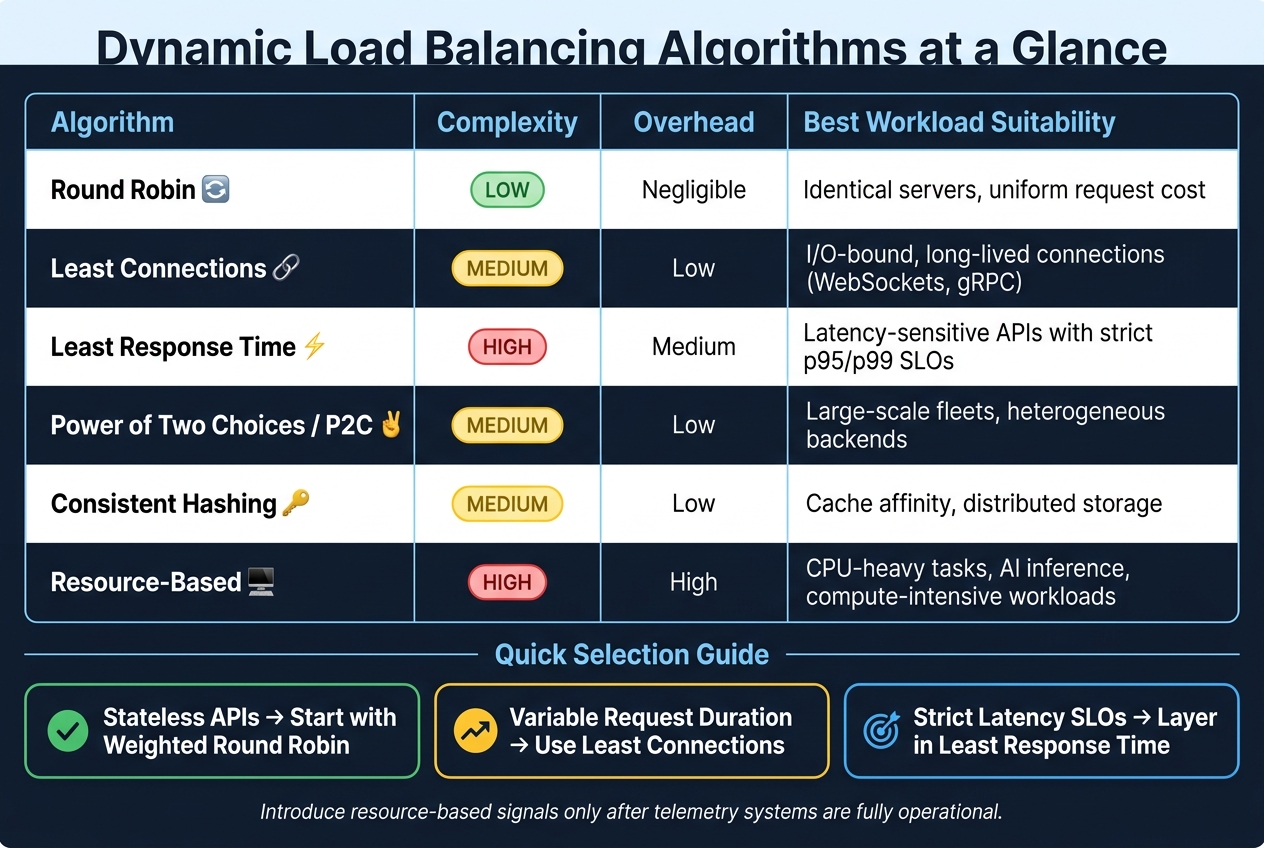
Algorithm	Complexity	Overhead	Best Workload Suitability
Round Robin	Low	Negligible	Identical servers, uniform request cost
Least Connections	Medium	Low	I/O-bound, long-lived connections (e.g., WebSockets, gRPC)
Least Response Time	High	Medium	Latency-sensitive APIs with strict p95/p99 SLOs
Power of Two (P2C)	Medium	Low	Large-scale fleets, heterogeneous backends
Consistent Hashing	Medium	Low	Cache affinity, distributed storage
Resource-Based	High	High	CPU-heavy tasks, AI inference, compute-intensive workloads

For stateless APIs, start with Weighted Round Robin. If your requests vary in duration, Least Connections is a better option. When latency targets become critical, layer in response-time weighting, and only introduce resource-based signals once your telemetry systems are fully operational.

Integrating Auto-Scaling with Dynamic Load Balancing

Managing traffic effectively goes beyond just balancing the load; it’s about ensuring your infrastructure keeps up with demand. When traffic spikes hit - whether it’s from a viral tweet, a Black Friday rush, or even a sudden bot attack - your load balancer needs more than smart routing. It needs an infrastructure that can expand and contract dynamically. That’s where auto-scaling comes in, adjusting resources in real time to handle the ebb and flow of demand.

"Traffic spikes do not send calendar invites. Your Black Friday sale, viral tweet, or unexpected bot attack will arrive without warning, and your infrastructure needs to scale before users start seeing 503 errors." - Nawaz Dhandala, OneUptime

For this integration to work smoothly, three key components must come together: a metrics collection layer (tracking CPU usage, request rate, and latency), a decision engine to evaluate thresholds, and a resource provisioner to allocate resources and update the load balancer’s configuration. Neglect any one of these, and the system won’t function as intended.

Health Checks and Service Discovery

The reliability of your load balancer’s routing depends entirely on the health signals it receives. Kubernetes employs two types of probes for this: liveness probes, which detect and restart crashed or stuck processes, and readiness probes, which ensure a pod is ready to handle traffic. To avoid directing traffic to shutting-down pods, readiness probes and PreStop hooks are essential. These mechanisms help prevent errors like 504s during scale-down events. Additionally, registering pods as IP targets can eliminate unnecessary network hops, providing direct and accurate health feedback.

Dynamic Scaling with Load Balancers

With health checks in place, your load balancer can drive dynamic scaling decisions. Kubernetes’ Horizontal Pod Autoscaler (HPA) operates on a 15-second sync cycle by default. While CPU and memory metrics are common triggers, they’re not always the best indicators. These metrics tend to lag behind actual demand, which means by the time CPU usage spikes, the traffic surge is already underway.

"Traffic is a leading indicator that represents instantaneous demand compared with CPU or memory which are lagging indicators." - Google Cloud Documentation

A more proactive approach involves using Requests Per Second (RPS) from the load balancer to inform the autoscaler. Setting a maxRatePerEndpoint can also help the load balancer identify when a service has reached capacity, prompting either local scaling or redirecting traffic to another cluster or region. For event-driven workloads, such as message queues or asynchronous job processors, KEDA (Kubernetes Event-driven Autoscaling) can adjust pod counts based on queue depth or Prometheus metrics. Unlike HPA, KEDA can even scale pods down to zero when there’s no demand.

For example, in January 2026, developer Sergio Sediq deployed a microservices architecture on AWS EKS. Using HPA, he configured scaling between 3 and 15 pods per service, triggered by CPU usage exceeding 70% or memory usage over 80%. This setup ensured a 2–3 minute scale-up time and maintained 100% availability across three availability zones during peak loads.

Avoiding Common Scaling Problems

Even with auto-scaling, challenges like oscillation can arise. Oscillation happens when the autoscaler scales up, causing metrics to drop, then scales down, only for metrics to climb again, leading to a cycle of instability. Kubernetes mitigates this with a 300-second stabilisation window for scale-down events, which ensures decisions are based on the most conservative scaling recommendation during that time. The rule is simple: scale up quickly, but scale down gradually.

Cold starts are another issue to watch out for. For instance, Java services often consume high CPU during startup due to JIT compilation. If the autoscaler misinterprets these spikes as actual load, it might over-provision resources unnecessarily. Using startupProbes can help the autoscaler ignore this initialisation phase, and readiness probes should only signal Ready once the service is fully operational. For latency-sensitive applications, deploying low-priority "pause" pods can provide an instant buffer. These pods can be quickly evicted to free up capacity when a real traffic surge occurs.

Lastly, always enable connection draining on your load balancer. This ensures that when pods are removed during scale-down, in-flight requests are allowed to complete instead of being dropped. Skipping this step can lead to unnecessary errors during routine scaling operations.

Monitoring, Testing, and Tuning Load Balancing

After implementing auto-scaling and health checks, the next step is to ensure your load balancing performs efficiently and to address potential issues before they affect users.

Key Metrics and Observability Tools

When deciding what to monitor, two popular frameworks stand out. The RED methodology focuses on three key signals for microservices: Rate (requests per second), Errors (failed requests), and Duration (how long requests take). On the other hand, Google’s Four Golden Signals include Latency, Traffic, Errors, and Saturation (how close a service is to hitting its resource limits). Both approaches help identify performance bottlenecks, but there’s more to monitor.

A healthy load balancer distributes requests evenly across all instances. To measure this, calculate the Coefficient of Variation (standard deviation divided by the average). A value below 0.1 indicates good balance, while anything above 0.3 suggests uneven distribution. For systems using long-lived connections, it’s better to track active connections per endpoint instead of raw request counts.

"A spike in p99 latency can indicate a serious problem even when the average looks fine." - Microservices Monitoring Guide

Latency is another critical metric. Track p50, p95, and p99 latencies, aiming for a p95 under 500 ms and keeping error rates below 0.1%. Set alerts for resource usage: warnings at 80% CPU or memory utilisation and critical alerts at 95%. For latency, trigger warnings when p99 exceeds 1 second and critical alerts when it surpasses 3 seconds.

For instrumentation, OpenTelemetry (OTel) is the go-to standard. It allows you to collect data once and send it to any backend, such as Jaeger, Prometheus, or Grafana. Tools like Kiali can visualise traffic flow, highlighting issues with red edges for errors and thicker edges for heavier traffic. While open-source solutions like Prometheus and Grafana are powerful, they often require more effort to manage compared to commercial tools like Datadog.

These metrics and tools form the foundation for testing and refining your load balancing setup.

Load Testing and Chaos Engineering

Understanding your metrics is essential, but testing your system under stress ensures it performs under real-world conditions. Replay actual production traces in a staging environment to see how the algorithm handles realistic traffic patterns. This approach can uncover hidden issues, such as uneven request costs.

Error injection is another valuable technique. Simulate backend problems like latency spikes or intermittent 5xx errors to see how algorithms like Least Response Time or Power of Two Choices (P2C) adjust traffic distribution. Additionally, test node churn by adding and removing instances during a run. This helps you evaluate how well the system handles session affinity and cache disruptions.

"Many production outages blamed on 'capacity' were really caused by naive traffic distribution interacting badly with autoscaling and slow starting instances." - Kelsey Hightower, Former Staff Engineer, Google

Before running chaos experiments, define abort thresholds. For example, stop the test if p95 latency increases by 20% for 10 minutes or if the error rate rises by 1.5× the baseline. During tests, compare the requests routed to each backend with those successfully completed. If a node gets its usual share of requests but completes fewer, it may indicate a hidden failure the load balancer is masking.

Once testing is complete, use the results to fine-tune your load balancing setup.

Tuning Parameters and Cutting Costs

Start by analysing your metrics, then adjust load balancing algorithms and scaling thresholds together. Changing one without the other can lead to inaccurate results. In environments with mixed instance types, algorithms like Weighted Round Robin or Least-Time routing can direct more traffic to higher-performance instances, making better use of premium resources.

Health check sensitivity is another key factor. Set intervals between 5–30 seconds and require two to three consecutive failures before removing an endpoint. This strikes a balance between fault tolerance and avoiding premature removals. Use a combination of passive health checks and active probes to quickly detect sudden issues.

For predictable traffic patterns, scheduled scaling can optimise costs. For instance, if traffic peaks during business hours, pre-scale your infrastructure to handle the load and scale down during off-peak times. This approach reduces reliance on reactive triggers and ensures that capacity matches demand. Setting clear minimum and maximum capacity limits further aligns costs with actual usage.

"Autoscaling transforms your infrastructure from a fixed cost to a variable cost that matches demand." - Nawaz Dhandala, Author, OneUptime

Conclusion

Dynamic load balancing remains a challenging yet essential task as microservices architectures continue to develop. With the global microservices market expected to hit around £13 billion by 2030, it’s clear that microservices are becoming a cornerstone of modern software development. This makes effective load balancing a critical focus for ensuring scalable and resilient systems.

"Intelligent load balancing is not just about distributing requests - it's about enabling modern, resilient architectures that can adapt to change in real time." - Muhammad Raza, Technology Writer

One crucial takeaway from this guide is that fairness in distributing requests doesn’t necessarily equate to fairness in actual workload. Algorithms like Power of Two Choices, Least Response Time, and Weighted Round Robin all have their strengths, but none are sufficient on their own. They must work hand-in-hand with service discovery, thorough health checks, and real-time observability to achieve reliable results.

Dynamic capacity estimation has shown the potential to significantly enhance performance, improving response time distribution by 200–400% and cutting tail latency by 50%. Such outcomes are far beyond what static configurations can achieve.

Key practices to keep in mind include:

• Using readiness probes alongside liveness checks to ensure accurate instance health monitoring
• Gradually ramping up traffic to new instances over 30–120 seconds to avoid sudden spikes
• Externalising session state to eliminate sticky-session limitations
• Monitoring p95 and p99 latencies for a more accurate view of performance, rather than relying on averages

As highlighted earlier, dynamic load balancing is not about a single solution but a combination of algorithms, health checks, and observability working together. Research consistently shows that no single algorithm excels in every scenario. The best approach depends on your specific workload, instance setup, and traffic patterns. Think of your load balancing configuration as a dynamic part of your infrastructure - one that requires regular versioning, testing, and refinement, just like your application code.

FAQs

Which load-balancing algorithm should I start with for my microservice?

The ideal load-balancing algorithm hinges on your service's request patterns and how consistent your resources are. For straightforward microservices handling uniform, short-lived requests, Round Robin offers a straightforward and predictable approach. If your servers have differing capacities, Weighted Round Robin adjusts accordingly. For workloads with a mix of requests or long-lived connections, Least Connections helps avoid overloading any single node. Antler Digital leverages these methods to design scalable and high-performing systems.

Where should load balancing live: edge, mesh, or client-side?

In microservices architecture, a hybrid model often works best. An edge load balancer handles incoming traffic, manages TLS termination, and performs routing tasks. Meanwhile, for internal service-to-service communication, a service mesh equipped with sidecar proxies offers dynamic and precise load balancing. This setup ensures robust perimeter security while enabling efficient, container-aware routing within the system.

What metrics should I use to drive autoscaling and routing?

For managing autoscaling and routing in microservices efficiently, keep an eye on resource usage and application-specific metrics. Important indicators to track include CPU and memory usage, request latency, error rates, and throughput. For more precise control, consider monitoring factors like queue depth, database connection pool activity, and tailored metrics such as RabbitMQ queue length. These real-time data points help ensure dynamic routing, minimise cascading failures, and align scaling actions with the actual workload.